Analytical Mapping

Loading packages and importing dataset

pacman::p_load(sf, tmap, tidyverse)

NGA_wp <- read_rds("rds/NGA_wp.rds")

Plotting the choropleth map

p1 <- tm_shape(NGA_wp) +
  tm_fill("wp_functional",
          n = 10,
          style = "equal",
          palette = "BuPu") +
  tm_borders(lwd = 0.1,
             alpha = 1) +
  tm_layout(main.title = "Distribution of functional water point by LGAs",
            legend.outside = FALSE)

p2 <- tm_shape(NGA_wp) +
  tm_fill("total_wp",
          n = 10,
          style = "equal",
          palette = "BuPu") +
  tm_borders(lwd = 0.1,
             alpha = 1) +
  tm_layout(main.title = "Distribution of total  water point by LGAs",
            legend.outside = FALSE)

tmap_arrange(p2, p1, nrow = 1)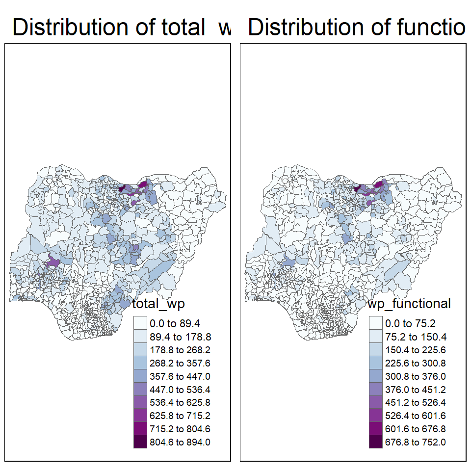

Mapping Rates (Proportions)

First, derive the percentages in the table.

NGA_wp <- NGA_wp %>%
  mutate(pct_functional = wp_functional/total_wp) %>%
  mutate(pct_nonfunctional = wp_nonfunctional/total_wp)

Plot the map:

p3 <- tm_shape(NGA_wp) +
  tm_fill("pct_functional",
          n = 10,
          style = "equal",
          palette = "BuPu") +
  tm_borders(lwd = 0.1,
             alpha = 1) +
  tm_layout(main.title = "Distribution of functional water point by LGAs",
            legend.outside = TRUE)

p3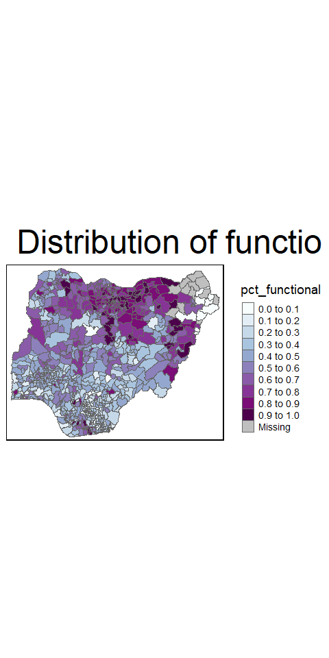

Extreme value maps

These are variations of common choropleth maps where the classification is designed to highlight extreme values at the lower and upper end of the scale, with the goal of identifying outliers.

Percentile maps

The percentile map is a special type of quantile map with six specific categories: 0-1%,1-10%, 10-50%,50-90%,90-99%, and 99-100%. The corresponding breakpoints can be derived by means of the base R quantile command, passing an explicit vector of cumulative probabilities as c(0,.01,.1,.5,.9,.99,1). Note that the begin and endpoint need to be included.

Prep the data:

NGA_wp <- NGA_wp %>%
  drop_na()

percent <- c(0,.01,.1,.5,.9,.99,1)
var <- NGA_wp["pct_functional"] %>%
  st_set_geometry(NULL)
quantile(var[,1], percent)

       0%        1%       10%       50%       90%       99%      100% 
0.0000000 0.0000000 0.2169811 0.4791667 0.8611111 1.0000000 1.0000000 

(Note: st_set_geometry(NULL) is used to drop the geometry field so that base r doesn’t struggle with it when extracting variables.)

Creating the get.var function

get.var <- function(vname,df) {
  v <- df[vname] %>% 
    st_set_geometry(NULL)
  v <- unname(v[,1])
  return(v)
}

A percentile mapping function

percentmap <- function(vnam, df, legtitle=NA, mtitle="Percentile Map"){
  percent <- c(0,.01,.1,.5,.9,.99,1)
  var <- get.var(vnam, df)
  bperc <- quantile(var, percent)
  tm_shape(df) +
  tm_polygons() +
  tm_shape(df) +
     tm_fill(vnam,
             title=legtitle,
             breaks=bperc,
             palette="Blues",
          labels=c("< 1%", "1% - 10%", "10% - 50%", "50% - 90%", "90% - 99%", "> 99%"))  +
  tm_borders() +
  tm_layout(main.title = mtitle, 
            title.position = c("right","bottom"))
}

Run them:

percentmap("total_wp", NGA_wp)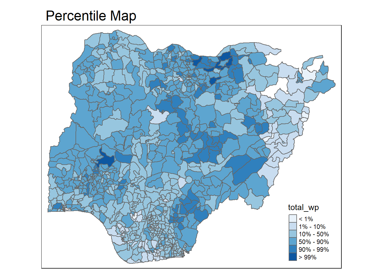

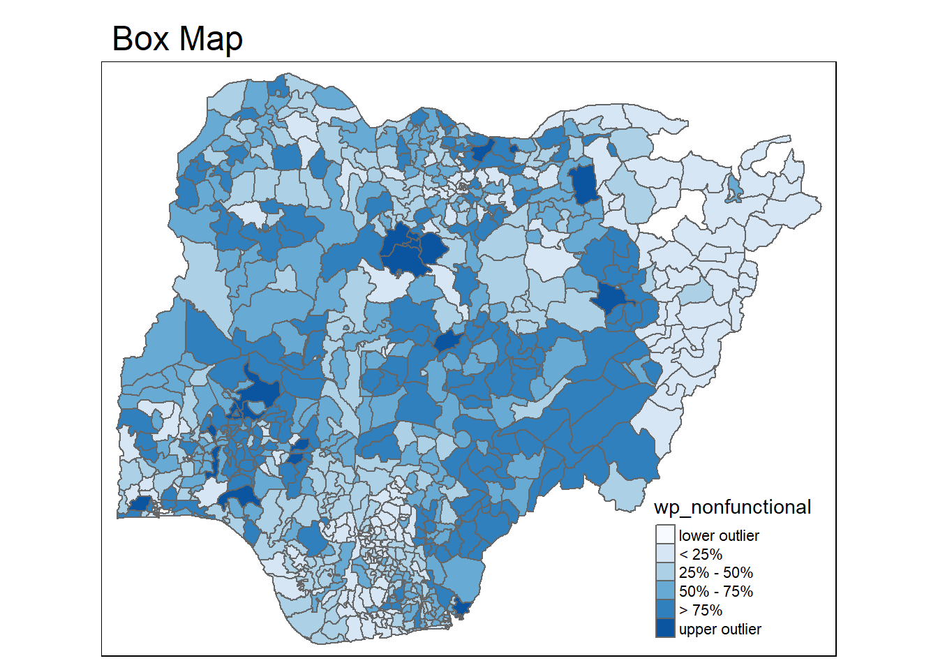
Box maps

A box map is an augmented quartile map, with an additional lower and upper category. When there are lower outliers, then the starting point for the breaks is the minimum value, and the second break is the lower fence. In contrast, when there are no lower outliers, then the starting point for the breaks will be the lower fence, and the second break is the minimum value (there will be no observations that fall in the interval between the lower fence and the minimum value).

ggplot(data = NGA_wp,
       aes(x = "",
           y = wp_nonfunctional)) +
  geom_boxplot()

Creating the boxbreaks function

Arguments:

• v : vector with observations

• mult : multiplier for inter-quartile range (default is 1.5)

Returns:

• bb: vector with 7 break points compute quartile and fences

boxbreaks <- function(v,mult=1.5) {
  qv <- unname(quantile(v))
  iqr <- qv[4] - qv[2]
  upfence <- qv[4] + mult * iqr
  lofence <- qv[2] - mult * iqr
  # initialize break points vector
  bb <- vector(mode="numeric",length=7)
  # logic for lower and upper fences
  if (lofence < qv[1]) {  # no lower outliers
    bb[1] <- lofence
    bb[2] <- floor(qv[1])
  } else {
    bb[2] <- lofence
    bb[1] <- qv[1]
  }
  if (upfence > qv[5]) { # no upper outliers
    bb[7] <- upfence
    bb[6] <- ceiling(qv[5])
  } else {
    bb[6] <- upfence
    bb[7] <- qv[5]
  }
  bb[3:5] <- qv[2:4]
  return(bb)
}

Creating the get.var function

get.var <- function(vname,df) {
  v <- df[vname] %>% st_set_geometry(NULL)
  v <- unname(v[,1])
  return(v)
}

Run it:

var <- get.var("wp_nonfunctional", NGA_wp) 
boxbreaks(var)

[1] -56.5   0.0  14.0  34.0  61.0 131.5 278.0

The Boxmap function

boxmap <- function(vnam, df, 
                   legtitle=NA,
                   mtitle="Box Map",
                   mult=1.5){
  var <- get.var(vnam,df)
  bb <- boxbreaks(var)
  tm_shape(df) +
    tm_polygons() +
  tm_shape(df) +
     tm_fill(vnam,title=legtitle,
             breaks=bb,
             palette="Blues",
          labels = c("lower outlier", 
                     "< 25%", 
                     "25% - 50%", 
                     "50% - 75%",
                     "> 75%", 
                     "upper outlier"))  +
  tm_borders() +
  tm_layout(main.title = mtitle, 
            title.position = c("left",
                               "top"))
}

tmap_mode("plot")
boxmap("wp_nonfunctional", NGA_wp)